In Google Sheets Can I Unhide and Then Hide Multiple Rows Again
There are different ways to hide and unhide rows or columns in Google Sheets.
The unhiding of rows or columns depends on different aspects. I mean, start, y'all must know the way the rows or columns are got subconscious. And so y'all tin retrieve nigh unhiding.
There are 3 different methods actually. I'll elaborate on each one of them.
This tutorial is especially for beginners. I may write a few more tutorials in this kind. Here nosotros become!
Iii Options to Hide and Unhide Rows or Columns and Benefits
When y'all only want to hide rows or columns in Google Sheets, use option # 1 beneath.
If y'all want to hibernate a bunch of rows or columns that need to hide and unhide often, then the better method in Google Sheets is option # 2 below.
Choice # iii is for conditionally hiding rows (not columns).
Choice one – Hide and Unhide Rows and Columns in the Normal Mode in Google Sheets
How to Hibernate and Unhide Bordering and Distant Columns in Google Sheets
Hide Columns:
This is the simplest and widely pop method to hide rows or columns in Google Sheets. If yous are using a desktop or laptop computer, you can follow the below method to hide columns in Google Sheets.
Assume you want to hibernate the adjoining columns F, G, and H. So follow the beneath ii steps.
- Select the columns to hide. How?
- Outset click on column letter F, press and hold the Shift central and click on cavalcade alphabetic character H.
- And then correct-click and select 'Hibernate columns F – H'.
If you want to hide distant columns, for example, column F and H just, the use Ctrl central instead of Shift.
I mean, select the first column, then press and hold the Ctrl key and click on some other column.
Unhide Columns:
To unhide adjoining columns, a single column, or distant columns in Google Sheets refer to the below screenshot. Please pay your attending to the arrow key which used for unhiding the columns.

How to Unhide All the Hidden Columns in a Flash in Google Sheets?
Offset and foremost, select the entire columns. How?
To do that click on the first column letter A, and then press Ctrl+Shift fundamental multiple (twice) times. And then correct-click and select 'Unhide columns'.
This manner you can hide/unhide columns in Google Sheets.
Hide Adjoining and Distant Rows
Hide Rows:
Every bit an example, to hide the adjoining rows 3 to 5, click on row # 3, press and hold the shift fundamental, and then click on row # four.
Right-click and choose 'Hide rows 3 – 5' to hide the bordering rows three to v in Google Sheets.
To hide distant rows, use the Ctrl cardinal instead of the Shift fundamental.
Unhide Rows:
Follow the below method (screenshot) to unhide, adjoining rows, a single row, or distant rows in Google Sheets.
How to Unhide All the Hidden Rows in a Flash in Google Sheets?
To unhide all the hidden rows in a flash, select all the rows in the sheet and so right-click and choose 'Unhide rows'.
Annotation
After selecting the columns or rows, you can also perform the above actions (hiding/unhiding of rows/columns), using shortcut keys.
Become to the Assist carte within your sheet and select 'Keyboard shortcuts. Search 'hide' and hit enter to notice the supporting shortcuts.
If you ask me about the benefit/pros of this method (Selection # one), let me say, it is the simplest method to hide/unhide random rows and columns in Google Sheets.
Option ii – Hide and Unhide Rows or Columns Using Group Command in Google Sheets
Here is some other mode to hide/unhide rows or columns in Google Sheets.
Grouping is the all-time way to hide and unhide a bunch of rows in Google Sheets. That's the benefit of using this option.
I'll explain where y'all will find this pick useful in real life.
Columns
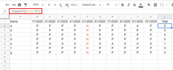
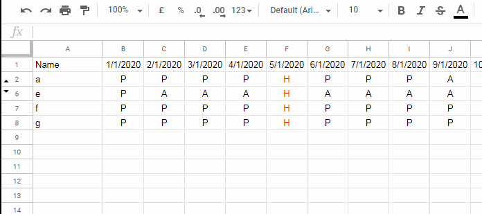
In the higher up example, cavalcade A contains names of students, and columns B to Yard contain their present and absent status.
Using the beneath COUNTIF in cell L2 which then dragged to cell L8, I take counted the full "P" (present) of each student.
=countif(B2:K2,"P") I merely don't want to see cavalcade B to K always. How to hide and unhide the columns B to K using the Data menu Group feature? Here are the steps.
- Select columns to B to 1000.
- Right-click and select 'Group columns B – K.
- Then click on the
-button to hibernate the columns and+button to unhide the columns. It's actually chosen collapse and expand column group.
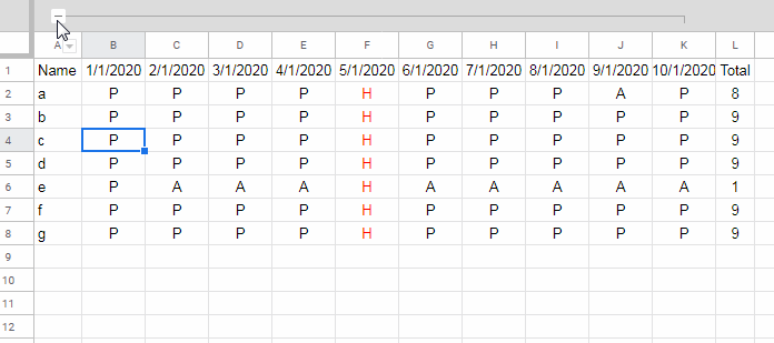
To entirely remove the group, correct-click anywhere on the group bar (the directly line on the tiptop) and select the 'Remove group' command.
Rows
Here I am non repeating the whole steps again. Just follow the above column grouping to hide and unhide a bunch of rows.
Instead of columns, hither select rows, and group rows. Further here are some avant-garde tutorial related grouping of rows.
- How to Group Rows and Columns in Google Sheets.
- Get Total Only When Group | Subgroup Is Collapsed in Google Sheets.
- Grouping and Subtotal in Google Sheets and Excel.
Selection 3 – Using Create a Filter Command
Using the data bill of fare 'Create a filter' nosotros can conditionally hibernate rows in Google Sheets (benefit/pros). It's just for rows (cons).
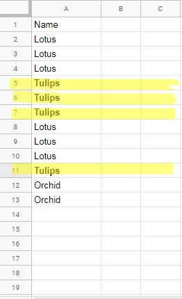
In the beneath example, I want to hide and unhide the rows containing 'Tulips'. How to do that using the 'Create a filter' menu command in Google Sheets?
Steps:
- Select the range A1:A13 or in example you want to include hereafter rows in the filter, select unabridged column A.
- Go to Data > Create a filter.
- It'll exit a drop-downwardly carte du jour icon in the very offset cell in the range, here it is in cell A1.
- Click it and remove the tick mark against 'Tulips' and click OK.
This will hide the rows containing 'Tulips'.
To unhide get to the drop-downwardly again and make a tick mark against 'Tulips' or click on Data > turn off the filter.
Filter Menu – Resource
- How to Filter by Calendar month Using the Filter Bill of fare in Google Sheets.
- Filter Unique Values Using the Filter Bill of fare in Google Sheets.
- Using Cell Reference in Filter Bill of fare Filter by Condition in Google Sheets.
- Filter by Date Range Using Filter Carte in Google Sheets.
- Filter Menu to Filter Max N Values in Google Sheets – Custom Formula.
In Google Sheets Can I Unhide and Then Hide Multiple Rows Again
Source: https://infoinspired.com/google-docs/spreadsheet/different-ways-hide-unhide-rows-columns-in-google-sheets/